上一节我们对数据集进行了初步的探索,并将其可视化,对数据有了初步的了解。这样我们有了之前数据探索的基础之后,就有了对其建模的基础feature,结合目标变量,即可进行模型训练了。我们使用交叉验证的方法来判断线下的实验结果,也就是把训练集分成两部分,一部分是训练集,用来训练分类器,另一部分是验证集,用来计算损失评估模型的好坏。
在Kaggle的希格斯子信号识别竞赛中,XGBoost因为出众的效率与较高的预测准确度在比赛论坛中引起了参赛选手的广泛关注,在1700多支队伍的激烈竞争中占有一席之地。随着它在Kaggle社区知名度的提高,最近也有队伍借助XGBoost在比赛中夺得第一。其次,因为它的效果好,计算复杂度不高,也在工业界中有大量的应用。
今天,我们就先来跑一个XGBoost版的Base Model。先回顾一下XGBoost的原理吧:机器学习算法系列(8):XgBoost
一、 准备工作
首先我们导入需要的包:
|
|
其中一些包的用途会在之后具体用到的时候进行讲解。
导入我们的数据:
|
|
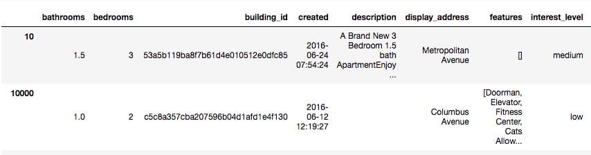
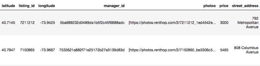
查看一下前两行:
|
|
二、特征构建
我们不需要对数值型数据进行任何的预处理,所以首先建立一个数值型特征的列表,纳入features_to_use
|
|
现在让我们根据已有的一些特征来构建一些新的特征:
|
|
我们有四个分类型的特征:
- display_address
- manager_id
- building_id
- street_address
可以对它们分别进行特征编码:
|
|
还有一些字符串类型的特征,可以先把它们合并起来
|
|
得到的字符串结果如下:
10000 Doorman Elevator Fitness_Center Cats_Allowed D…
100004 Laundry_In_Building Dishwasher Hardwood_Floors…
然后CountVectorizer类来计算TF-IDF权重
|
|
这里我们需要提一点,对数据集进行特征变换时,必须同时对训练集和测试集进行操作。现在把这些处理过的特征放到一个集合中(横向合并)
|
|
然后把目标变量转换为0、1、2,如下
|
|
可以看到,经过上面一系列的变量构造之后,其数量已经达到了217个。
接下来就可以进行建模啦。
三、XGB建模
先写一个通用的XGB模型的函数:
|
|
函数返回的是预测值和模型。
5折交叉验证将训练集划分为五份,其中的一份作为验证集。
|
|
结果如下:
|
|
迭代357次之后,在训练集上的对数损失为0.352182,在验证集上的损失为0.5478。
然后在对测试集进行预测:
|
|
把结果按照比赛规定的格式写入csv文件:
|
|
看一下最后的结果: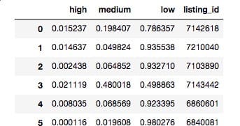
提交到kaggle上,这样我们整个建模的过程就完成了。
接下来两节中,我们重点讲一讲关于XGBoost的调参经验以及使用SK-learn计算TF-IDF。

